MMA Atoms in CuTe
Introduction
MMA Atoms are fundamental building blocks of CuTe kernels and therefore have a dedicated section in the CuTe docs as well. In this blogpost we offer a different angle on the same topic taking a different "route of explanation". For better understanding we take one of the examples that is used in the CuTe docs as well.
Understanding MMA Atoms
The following program will print a LaTeX file to the screen that can be in turn used to generate a visualization of the MMA Atom.
#include <cute/tensor.hpp>

int main() {
    using namespace cute;

    MMA_Atom mma = MMA_Atom<SM70_8x8x4_F32F16F16F32_NT>{};
    print_latex(mma);
    return 0;
}
To make sense of this it is useful to first look at the code:
In cutlass/include/cute/arch/mma_sm70.hpp we can find:
struct SM70_8x8x4_F32F16F16F32_NT
{
  using DRegisters = float[8];
  using ARegisters = uint32_t[2];
  using BRegisters = uint32_t[2];
  using CRegisters = float[8];

  // Register asm fma
  CUTE_HOST_DEVICE static void
  fma(float         & d0, float         & d1, float      & d2, float      & d3,
      float         & d4, float         & d5, float      & d6, float      & d7,
      uint32_t const& a0, uint32_t const& a1,
      uint32_t const& b0, uint32_t const& b1,
      float    const& c0, float    const& c1, float const& c2, float const& c3,
      float    const& c4, float    const& c5, float const& c6, float const& c7)
  {
#if defined(CUTE_ARCH_MMA_SM70_ENABLED)
    asm volatile("mma.sync.aligned.m8n8k4.col.row.f32.f16.f16.f32"
                 "{%0,  %1,  %2,  %3,  %4,  %5,  %6,  %7},"
                 "{%8,  %9},"
                 "{%10, %11},"
                 "{%12, %13, %14, %15, %16, %17, %18, %19};"
        : "=f"(d0), "=f"(d1), "=f"(d2), "=f"(d3),
          "=f"(d4), "=f"(d5), "=f"(d6), "=f"(d7)
        :  "r"(a0),  "r"(a1),
           "r"(b0),  "r"(b1),
           "f"(c0),  "f"(c1),  "f"(c2),  "f"(c3),
           "f"(c4),  "f"(c5),  "f"(c6),  "f"(c7));
#else
    CUTE_INVALID_CONTROL_PATH("Attempting to use SM70_8x8x4_F32F16F16F32_NT without CUTE_ARCH_MMA_SM70_ENABLED");
#endif
  }
};
We see that this essentially a wrapper around a PTX instruction which can be understood as follows:
mma.sync.aligned.m8n8k4.col.row.f32.f16.f16.f32

- A: 8 x 4 -> Float 16, column major
- B: 4 x 8 -> Float 16, row major (same as 8 x 4 in column major)
- C: 8 x 8 -> Float 32
- D: 8 x 8 -> Float 32
Looking at section 9.7.14.5.1 we see that 8 threads will perform one such MMA and that the values for A and B should be provided as a vector expression containing two .f16x2 registers.
This is exactly what we can see in the above PTX instruction which gets passed 8 * 8 / 8 = 8 values for D/C and 8 * 4 / 8 / 2 = 2 values for A/B.
In PTX docs we can furthermore find Layout for our MMA instruction. Note that PTX docs informs us that
Elements of 4 matrices need to be distributed across the threads in a warp. The following table shows distribution of matrices for MMA operations.
MMA computation 1: Threads 0-3, Threads 16-19
MMA computation 2: Threads 4-7, Threads 20-23
MMA computation 3: Threads 8-11, Threads 24-27
MMA computation 4: Threads 12-15, Threads 28-31
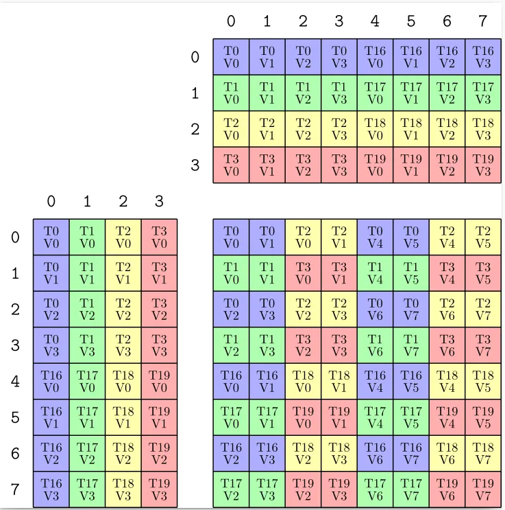
A Layout
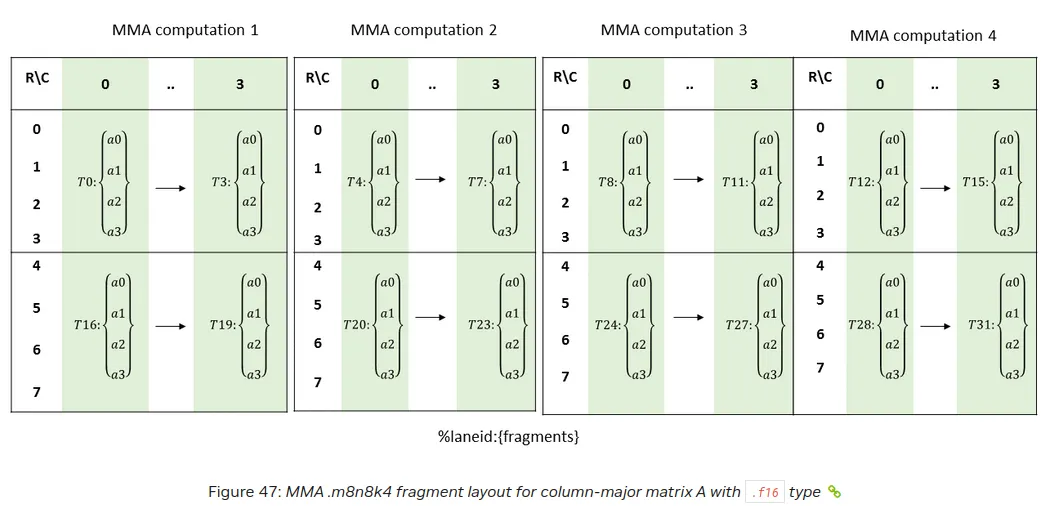
Note that the above picture for MMA computation 1 is equivalent to the situation we see above in our picture. We can derive the TV Layout:
To derive Thread Layout we note that it consists for one computation of 8 threads which can be split up into two groups. So we have two modes for the thread layout and need to derive the shapes and strides for each mode.
(T0, a0) -> (T1, a0)
takes 8 steps. We have 4 elements (T0, a0), (T1, a0), (T2, a0), (T3, a0) in this group.
(T0, a0) -> (T16, a0)
takes 4 steps. We have 2 elements (T0, a0), (T16, a0) in this group.
The value layout is simple because each thread has just 4 values which have a stride of 1 in between. This gives us ((4, 2), 4):((8,4),1) for the TV Layout of A.
B Layout
From the PTX docs:
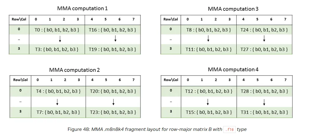
Unsurprisingly this again agrees with what we see above.
Note that equivalently we may interpret B has a 8 x 4 matrix in column major. To see why that is true consider:
1) M: N x K in column major
2) M^T K x N in row major

Coordinate mapping:
for (i, j) in {0, ..., N-1} x {0, ..., K-1}
(i, j) -> j * N + i
(j, i) -> j * N + i
We than can use same TV Layout as above for A.
C Layout
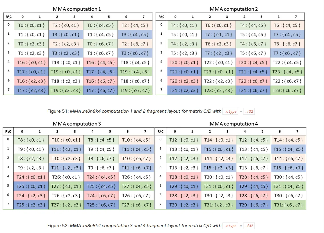
Once more we see that MMA computation 1 matches the above depiction.
Where do the Layouts come from?
In cutlass/include/cute/atom/mma_atom.hpp we find:
template <class MMAOperation>
struct MMA_Atom<MMAOperation> : MMA_Atom<MMA_Traits<MMAOperation>>
{};
in cutlass/include/cute/atom/mma_traits_sm70.hpp we find
namespace {
// Logical thread id to thread idx (quadpair)
using SM70_QuadPair = Layout<Shape <_4, _2>,
                             Stride<_1,_16>>;
// (T8,V4) -> (M8,K4)
using SM70_8x4_Row  = Layout<Shape <_8,_4>,
                             Stride<_1,_8>>;
// (T8,V4) -> (M8,K4)
using SM70_8x4_Col  = Layout<Shape <Shape <_4,_2>,_4>,
                             Stride<Stride<_8,_4>,_1>>;
// (T8,V8) -> (M8,N8)
using SM70_8x8_16b  = Layout<Shape <_8,_8>,
                             Stride<_1,_8>>;
// (T8,V8) -> (M8,N8)
using SM70_8x8_32b  = Layout<Shape <Shape <_2, _2,_2>,Shape <_2,_2, _2>>,
                             Stride<Stride<_1,_16,_4>,Stride<_8,_2,_32>>>;
}
...
template <>
struct MMA_Traits<SM70_8x8x4_F32F16F16F32_NT>
{
  using ValTypeD = float;
  using ValTypeA = half_t;
  using ValTypeB = half_t;
  using ValTypeC = float;

  using Shape_MNK = Shape<_8,_8,_4>;
  using ThrID   = SM70_QuadPair;
  using ALayout = SM70_8x4_Col;
  using BLayout = SM70_8x4_Col;
  using CLayout = SM70_8x8_32b;
};
we see that this is where the Layout information is hardcoded into the trait for the operation. Note that it although B has same TV Layout as A we display it's transpose above in the picture. We explained above why the two representations (i.e. 4 x 8 row major and 8 x 4 column major) are equivalent. Note that the trait also contains information about the value types of the matrices as well as the general problem shape. The ThrId is needed for mapping within one MMA computation group. Within one group we have a total of 8 threads. They are spitted into two groups and within each group we have a stride of 1 (from 0 to 1 etc) whereas to go from one group to the other we have a stride of 16 (from 0 to 16 etc).
Visualization
Code for visualization can be found in cutlass/include/cute/util/print_latex.hpp.
template <class LayoutC, class LayoutA, class LayoutB, class Tile_MNK,
          class TikzColorFn = TikzColor_TV>
CUTE_HOST_DEVICE
void
print_latex_mma(LayoutC const& C,         // (tid,vid) -> (m,n) coord
                LayoutA const& A,         // (tid,vid) -> (m,k) coord
                LayoutB const& B,         // (tid,vid) -> (n,k) coord
                Tile_MNK const& tile_mnk, // (M,N,K)
                TikzColorFn color = {})   // lambda(tid,vid) -> tikz color string
{
  CUTE_STATIC_ASSERT_V(rank(C) == Int<2>{});
  CUTE_STATIC_ASSERT_V(rank(A) == Int<2>{});
  CUTE_STATIC_ASSERT_V(rank(B) == Int<2>{});

  // Commented prints
  printf("%% LayoutC: "); print(C); printf("\n");
  printf("%% LayoutA: "); print(A); printf("\n");
  printf("%% LayoutB: "); print(B); printf("\n");
  // Header
  printf("\\documentclass[convert]{standalone}\n"
         "\\usepackage{tikz}\n\n"
         "\\begin{document}\n"
         "\\begin{tikzpicture}[x={(0cm,-1cm)},y={(1cm,0cm)},every node/.style={minimum size=1cm, outer sep=0pt}]\n\n");

  auto [M, N, K] = product_each(shape(tile_mnk));
  Tensor filled = make_tensor<bool>(make_shape(M, N, K));
  clear(filled);

  // C starting at 0,0
  for (int tid = 0; tid < size<0>(C); ++tid) {
    for (int vid = 0; vid < size<1>(C); ++vid) {
      auto [m, n] = C(tid, vid);
      if (not filled(m, n, 0)) {
        filled(m, n, 0) = true;
        printf("\\node[fill=%s] at (%d,%d) {\\shortstack{T%d \\\\ V%d}};\n",
               color(tid, vid),
               int(m), int(n),
               tid, vid);
      }
    }
  }
  // Grid
  printf("\\draw[color=black,thick,shift={(-0.5,-0.5)}] (%d,%d) grid (%d,%d);\n\n",
          0, 0, int(M), int(N));

  clear(filled);

  // A starting at 0,-K-1
  for (int tid = 0; tid < size<0>(A); ++tid) {
    for (int vid = 0; vid < size<1>(A); ++vid) {
      auto [m, k] = A(tid, vid);
      if (not filled(m, 0, k)) {
        filled(m, 0, k) = true;
        printf("\\node[fill=%s] at (%d,%d) {\\shortstack{T%d \\\\ V%d}};\n",
               color(tid, vid),
               int(m), int(k-K-1),
               tid, vid);
      }
    }
  }
  // Grid
  printf("\\draw[color=black,thick,shift={(-0.5,-0.5)}] (%d,%d) grid (%d,%d);\n\n",
         0, -int(K)-1, int(M), -1);
  // A labels
  for (int m =  0, k = -1; m < M; ++m) {
    printf("\\node at (%d,%d) {\\Large{\\texttt{%d}}};\n", m, int(k-K-1), m);
  }
  for (int m = -1, k =  0; k < K; ++k) {
    printf("\\node at (%d,%d) {\\Large{\\texttt{%d}}};\n", m, int(k-K-1), k);
  }

  clear(filled);

  // B starting at -K-1,0
  for (int tid = 0; tid < size<0>(B); ++tid) {
    for (int vid = 0; vid < size<1>(B); ++vid) {
      auto [n, k] = B(tid, vid);
      if (not filled(0, n, k)) {
        filled(0, n, k) = true;
        printf("\\node[fill=%s] at (%d,%d) {\\shortstack{T%d \\\\ V%d}};\n",
               color(tid, vid),
               int(k)-int(K)-1, int(n),
               tid, vid);
      }
    }
  }
  // Grid
  printf("\\draw[color=black,thick,shift={(-0.5,-0.5)}] (%d,%d) grid (%d,%d);\n\n",
         -int(K)-1, 0, -1, int(N));
  // B labels
  for (int n =  0, k = -1; n < N; ++n) {
    printf("\\node at (%d,%d) {\\Large{\\texttt{%d}}};\n", int(k-K-1), n, n);
  }
  for (int n = -1, k =  0; k < K; ++k) {
    printf("\\node at (%d,%d) {\\Large{\\texttt{%d}}};\n", int(k-K-1), n, k);
  }

  // Footer
  printf("\\end{tikzpicture}\n"
         "\\end{document}\n");
}
We see that
auto [n, k] = B(tid, vid);
...
printf("\\node[fill=%s] at (%d,%d) {\\shortstack{T%d \\\\ V%d}};\n",
               color(tid, vid),
               int(k)-int(K)-1, int(n),
               tid, vid);
so the Layout gives us (n, k) coordinate, but we display it in the equivalent view as (k, n) row major.
Conclusion
I hope this can serve as a helpful complementary guide to the CUTLASS explanation of MMA Atoms. The same principles of analysis can of course be applied to other MMA Atoms. If you like to exchange ideas on similar topics feel free to connect to me on Linkedin.