Intuition behind Hierarchical Layouts

13 Aug, 2025

Introduction

Layouts, especially nested ones, can seem difficult to newcomers to CuTe. Actually they can be easily understand if one connects them to visuals. In this short note I will describe how to do that.

Intuitive Understanding of Layouts

The following function can be used to see how linear indices are mapped to the hierarchical ND coordinates by a given CuTe layout.

@cute.jit
def print_crd_for_idx(shape, stride):
    layout = cute.make_layout(shape, stride=stride)
    cute.printf(layout)
    for idx in range(cute.size(shape)):
        crd = layout.get_hier_coord(idx)
        cute.printf("{} -> {}", idx, crd)

We will now analyse different ways of how to "lay out" elements in memory in different ways. This will hopefully give a better intuitive understanding of Layouts. Our focus will be on nested Layouts which may be the most difficult to understand on an intuitive level for a beginner to CuTe.

Lets consider the following arrangement of elements in memory along a cube:

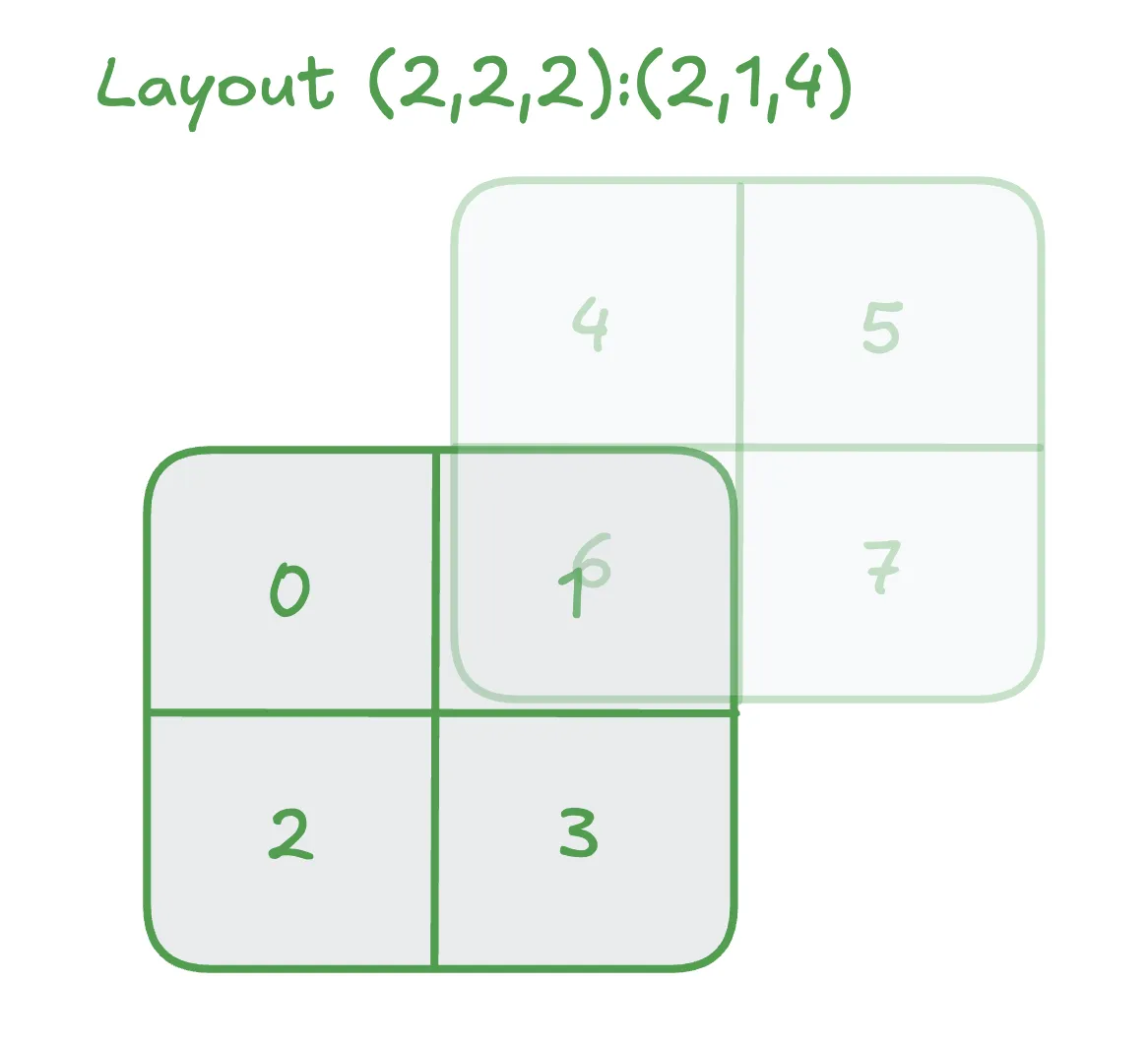
Note that we have two planes. The planes are K-Major, i.e. the stride along the first mode is 1 and the stride along the zeroth mode is 2. The stride between two planes is 4 which gives us (2,2,2):(2,1,4).

We can verify this via printing out the map:

(2,2,2):(2,1,4)
0 -> (0,0,0)
1 -> (0,1,0)
2 -> (1,0,0)
3 -> (1,1,0)
4 -> (0,0,1)
5 -> (0,1,1)
6 -> (1,0,1)
7 -> (1,1,1)

We may interpret this as a 4x2 matrix as follows:

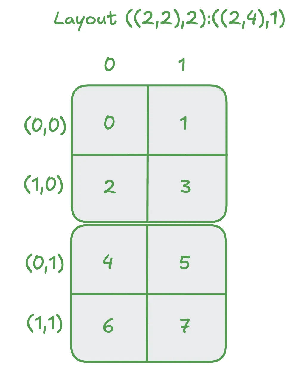
Note that here we use a 2d index for the zeroth mode. The stride can be easily read off as 2 in the zeroth mode of this sub layout and 4 in the first mode of this sub layout. The remaining stride (i.e. the one corresponding to the first mode of the full layout) is 1. This gives us ((2,2),2):((2,4),1) for the full layout.

The associated map confirms our understanding:

((2,2),2):((2,4),1)
0 -> ((0,0),0)
1 -> ((0,0),1)
2 -> ((1,0),0)
3 -> ((1,0),1)
4 -> ((0,1),0)
5 -> ((0,1),1)
6 -> ((1,1),0)
7 -> ((1,1),1)

We may also think of interpreting the above as a 2x4 matrix:

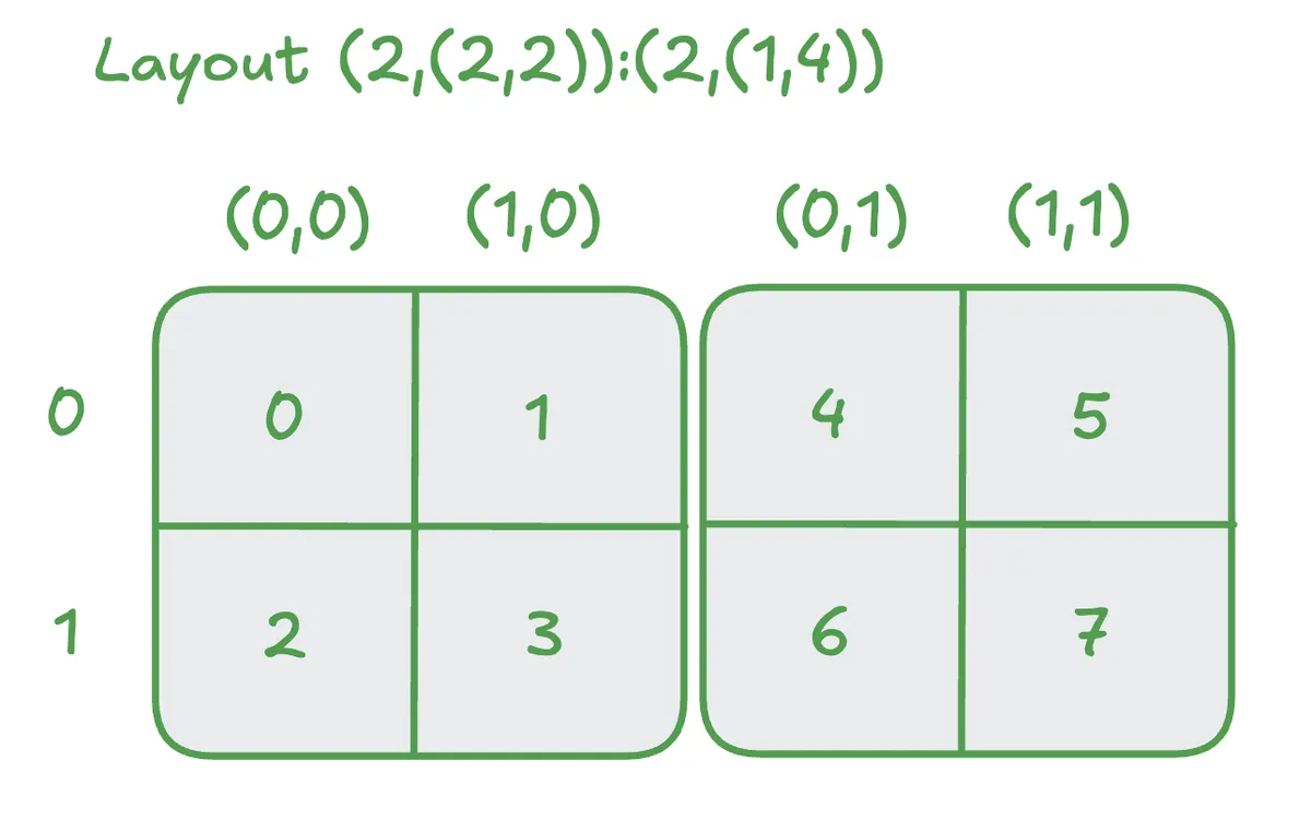
Note that here we have a 2d index in the first mode. We can read of the stride as 1 for the zeroth mode of this sub layout and 4 for the first mode of this sub layout. This is because from (0,0) -> (1,0) we make 1 step and from (0,0) -> (0,1) we make 4 steps. Similar we can read off the stride in the zeroth mode of the layout as 2. This gives us the full layout as (2,(2,2)):(2,(1,4)).

We can print out the map to confirm our understanding:

(2,(2,2)):(2,(1,4))
0 -> (0,(0,0))
1 -> (0,(1,0))
2 -> (1,(0,0))
3 -> (1,(1,0))
4 -> (0,(0,1))
5 -> (0,(1,1))
6 -> (1,(0,1))
7 -> (1,(1,1))

We can express even more complicated arrangements of the elements using the CuTe algebra:

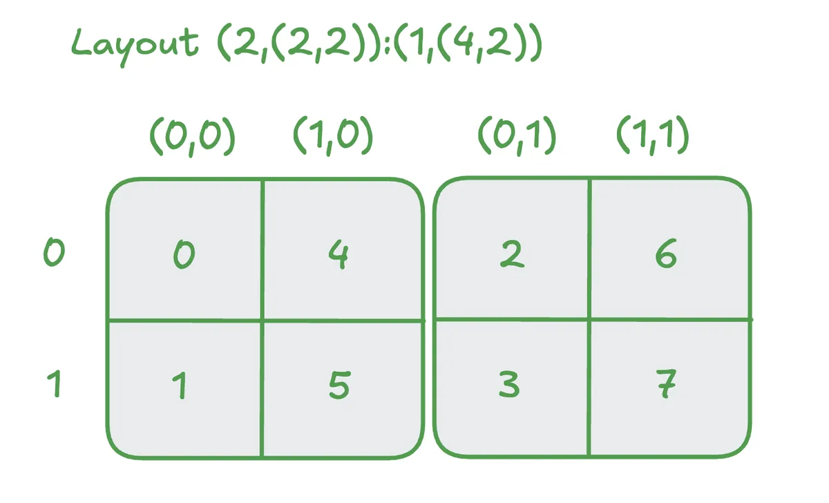
Note that here we have the sub layout (2,2):(4,2) for the first mode. We can see that the stride in the zeroth mode of this sub layout is 4, the stride in the first mode is 2. This is because to go from (0,0) -> (1,0) we need to make 4 steps and from (0,0) -> (0,1) we need to take 2 steps. The stride in the zeroth mode of the whole layout is 1.

This gives us the full layout as (2,(2,2)):(1,(4,2))

The map is given as:

(2,(2,2)):(1,(4,2))
0 -> (0,(0,0))
1 -> (1,(0,0))
2 -> (0,(0,1))
3 -> (1,(0,1))
4 -> (0,(1,0))
5 -> (1,(1,0))
6 -> (0,(1,1))
7 -> (1,(1,1))

We can even express very difficult patterns like the below quiet convenient using CuTe.

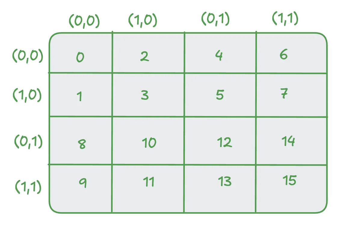
Let us derive this Layout by hand.

Let's first consider the sub layout for the zeroth mode. We can read it of as (2,2):(1,8). This can be seen in the picture above pretty clearly because from (0,0) -> (1,0) it takes one step and from (0,0) -> (0,1) it takes 8 steps.

Similar let us derive the other sub layout. We can read it off as (2,2):(2,4) with a similar reasoning like before. Let's confirm that this derivation was correct:

((2,2),(2,2)):((1,8),(2,4))
0 -> ((0,0),(0,0))
1 -> ((1,0),(0,0))
2 -> ((0,0),(1,0))
3 -> ((1,0),(1,0))
4 -> ((0,0),(0,1))
5 -> ((1,0),(0,1))
6 -> ((0,0),(1,1))
7 -> ((1,0),(1,1))
8 -> ((0,1),(0,0))
9 -> ((1,1),(0,0))
10 -> ((0,1),(1,0))
11 -> ((1,1),(1,0))
12 -> ((0,1),(0,1))
13 -> ((1,1),(0,1))
14 -> ((0,1),(1,1))
15 -> ((1,1),(1,1))

We see that it is very easy to express these complicated Layouts using CuTe once the mechanism is properly understood. This is very useful as Layouts expected of the Tensor Cores on NVIDIA GPUs can become quiet complicated as you can convince yourself in the PTX docs. In general indexing can be one of the main bottlenecks for productivity of the programmer. The CuTe Layouts let us express these indexing patters in an extremely intuitive and easy way. It is furthermore nice how easily we can express Layout coordinate mapping in the CuTeDSL. This gives us ability to analyse memory access patterns etc. in an easy way.

Conclusion

I hope this blogpost made Layouts and their interpretation more accessible. Feel free to connect with me if you like to exchange ideas via my Linkedin.