Chunkwise Gated Delta Rule

10 Mar, 2026

Chunkwise Gated Delta Rule is important when performing operations such as prefilling or training with the recently popular Gated Delta Attention formulation.

In essence, in the chunkwise algorithm, we want to transform the naive recurrent equations for the transition from one timestep to the next into a form that is more GPU-friendly. This works by splitting the sequence length into chunks and then deriving formulas to perform the transition from one chunk to the next via matrix multiplication. For Gated Delta Net, this is not completely straightforward, which is why I will derive the transition formulas step by step in this blog post. For educational purposes, we start with Linear Attention, then move to the Delta Rule, and finally to the Gated Delta Rule.

Chunkwise Linear Attention

S_{[t]}^{r} = S_{[t]} + \sum_{i = 1}^{r} v_{[t]}^{i} (k_{[t]}^{i})^{T} \in R^{d_{v} \times d_{k}}

where $v_{[t]}^{i} \in R^{d_{v} \times 1}$ denotes the i'th row relative to the beginning of the chunk $V_{t C + 1 : (t + 1) C} \in R^{C \times d_{v}}$ (we start to count from 1) of the matrix $V \in R^{L \times d_{v}}$ and similar for $K$ . $S_{[t]}$ is simply $S_{t C}$ and $S_{[t]}^{r}$ is this state shifted by $r$ timesteps.

For the output we have

o_{[t]}^{r} = S_{[t]}^{r} q_{[t]}^{r} = S_{[t]} q_{[t]}^{r} + \sum_{i = 1}^{r} v_{[t]}^{i} ((k_{[t]}^{i})^{T} q_{[t]}^{r}) \in R^{d_{v} \times 1}

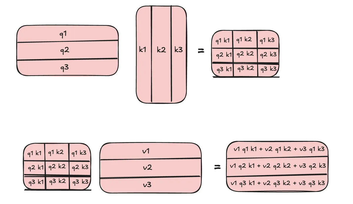
Note we can write this in matrix form as

S_{[t + 1]} = S_{[t]} + V_{[t]}^{T} K_{[t]} \in R^{d_{v} \times d_{k}}

and

O_{[t]} = Q_{[t]} S_{[t]}^{T} + (Q_{[t]} K_{[t]}^{T} ⊙ M) V_{[t]} \in R^{C \times d_{v}}

where $M \in R^{C \times C}$ is the causal mask. Why we need causal mask can be understood in a picture:

Causal Mask

But we see that the sum at timestep $r$ relative to beginning of chunk should just contain $r$ summands. This is achieved by causal masking which will eliminate all upper right entries from the matrix above and thus gives us $r$ summands for $r$ th row in second matrix.

Chunkwise Delta Rule

For Delta Rule we have state update as

S_{t} = S_{t - 1} (I - β_{t} k_{t} k_{t}^{T}) + β_{t} v_{t} k_{t}^{T} \in R^{d_{v} \times d_{k}}

As above we can expand the state by applying recursion to obtain the equation for an offset $r$ from the start of a chunk:

S_{[t]}^{r} = S_{[t]} \underset{: = P_{[t]}^{r}}{\underset{⏟}{(\prod_{i = 1}^{r} (I - β_{[t]}^{i} k_{[t]}^{i} (k_{[t]}^{i})^{T}))}} + \underset{: = H_{[t]}^{r}}{\underset{⏟}{\sum_{i = 1}^{r} (β_{[t]}^{i} v_{[t]}^{i} (k_{[t]}^{i})^{T} \prod_{j = i + 1}^{r} (I - β_{[t]}^{j} k_{[t]}^{j} (k_{[t]}^{j})^{T}))}} \in R^{d_{v} \times d_{k}} .

We will prove useful identity for these terms now.

$P_{[t]}^{r}$

Let's prove that

P_{[t]}^{r} = I - \sum_{i = 1}^{r} w_{[t]}^{i} (k_{[t]}^{i})^{T}

By induction over $r \in N_{> 0}$ .

$r = 1$ :

P_{[t]}^{1} = \prod_{i = 1}^{1} (I - β_{[t]}^{i} k_{[t]}^{i} (k_{[t]}^{i})^{T}) = I - β_{[t]}^{1} k_{[t]}^{1} (k_{[t]}^{1})^{T}

choose $w_{[t]}^{1} = β_{[t]}^{1} k_{[t]}^{1}$ and the equation is fulfilled.

$r \to r + 1$ :

For the induction step, we continue from

P_{[t]}^{r + 1} = P_{[t]}^{r} (I - β_{[t]}^{r + 1} k_{[t]}^{r + 1} (k_{[t]}^{r + 1})^{T})

and use the induction hypothesis

P_{[t]}^{r} = I - \sum_{i = 1}^{r} w_{[t]}^{i} (k_{[t]}^{i})^{T} .

Thus,

P_{[t]}^{r + 1} = (I - \sum_{i = 1}^{r} w_{[t]}^{i} (k_{[t]}^{i})^{T}) (I - β_{[t]}^{r + 1} k_{[t]}^{r + 1} (k_{[t]}^{r + 1})^{T}) .

Expanding the product yields

P_{[t]}^{r + 1} = I - β_{[t]}^{r + 1} k_{[t]}^{r + 1} (k_{[t]}^{r + 1})^{T} - \sum_{i = 1}^{r} w_{[t]}^{i} (k_{[t]}^{i})^{T} + \sum_{i = 1}^{r} w_{[t]}^{i} (k_{[t]}^{i})^{T} β_{[t]}^{r + 1} k_{[t]}^{r + 1} (k_{[t]}^{r + 1})^{T} .

Since $((k_{[t]}^{i})^{T} β_{[t]}^{r + 1} k_{[t]}^{r + 1})$ is a scalar, the last term can be rewritten as

\sum_{i = 1}^{r} β_{[t]}^{r + 1} ((k_{[t]}^{i})^{T} k_{[t]}^{r + 1}) w_{[t]}^{i} (k_{[t]}^{r + 1})^{T} .

Therefore,

P_{[t]}^{r + 1} = I - \sum_{i = 1}^{r} w_{[t]}^{i} (k_{[t]}^{i})^{T} - β_{[t]}^{r + 1} (k_{[t]}^{r + 1} - \sum_{i = 1}^{r} ((k_{[t]}^{i})^{T} k_{[t]}^{r + 1}) w_{[t]}^{i}) (k_{[t]}^{r + 1})^{T} .

Now define

w_{[t]}^{r + 1} : = β_{[t]}^{r + 1} (k_{[t]}^{r + 1} - \sum_{i = 1}^{r} ((k_{[t]}^{i})^{T} k_{[t]}^{r + 1}) w_{[t]}^{i}) .

Then we obtain

P_{[t]}^{r + 1} = I - \sum_{i = 1}^{r + 1} w_{[t]}^{i} (k_{[t]}^{i})^{T} .

This is exactly the desired form, so the induction step is proved.

Moreover, the proof gives a recursive way to compute the vectors $w_{[t]}^{r}$ : start with

w_{[t]}^{1} = β_{[t]}^{1} k_{[t]}^{1},

and for $r > 1$ compute

w_{[t]}^{r} = β_{[t]}^{r} (k_{[t]}^{r} - \sum_{i = 1}^{r - 1} ((k_{[t]}^{i})^{T} k_{[t]}^{r}) w_{[t]}^{i}) .

$H_{[t]}^{r}$

Let's prove that

H_{[t]}^{r} = \sum_{i = 1}^{r} u_{[t]}^{i} (k_{[t]}^{i})^{T}

By induction over $r \in N_{> 0}$ .

$r = 1$ :

H_{[t]}^{1} = \sum_{i = 1}^{1} (β_{[t]}^{i} v_{[t]}^{i} (k_{[t]}^{i})^{T} \prod_{j = i + 1}^{1} (I - β_{[t]}^{j} k_{[t]}^{j} (k_{[t]}^{j})^{T})) = β_{[t]}^{1} v_{[t]}^{1} (k_{[t]}^{1})^{T}

Choose $u_{[t]}^{1} = β_{[t]}^{1} v_{[t]}^{1}$ and the equation is fulfilled.

$r \to r + 1$ :

H_{[t]}^{r + 1} = \sum_{i = 1}^{r + 1} (β_{[t]}^{i} v_{[t]}^{i} (k_{[t]}^{i})^{T} \prod_{j = i + 1}^{r + 1} (I - β_{[t]}^{j} k_{[t]}^{j} (k_{[t]}^{j})^{T}))

Let's use the following identities to bring this into a form where we can use the induction hypothesis:

\sum_{j = 1}^{r + 1} x_{j} = (\sum_{j = 1}^{r} x_{j}) + x_{r + 1}

\prod_{j = 1}^{r + 1} x_{j} = (\prod_{j = 1}^{r} x_{j}) x_{r + 1}

Split up such that we first expand the last sum, and then the last product term for each product, and factor that out:

H_{[t]}^{r + 1} = \sum_{i = 1}^{r + 1} (β_{[t]}^{i} v_{[t]}^{i} (k_{[t]}^{i})^{T} \prod_{j = i + 1}^{r + 1} (I - β_{[t]}^{j} k_{[t]}^{j} (k_{[t]}^{j})^{T}))

= \sum_{i = 1}^{r} (β_{[t]}^{i} v_{[t]}^{i} (k_{[t]}^{i})^{T} \prod_{j = i + 1}^{r + 1} (I - β_{[t]}^{j} k_{[t]}^{j} (k_{[t]}^{j})^{T})) + β_{[t]}^{r + 1} v_{[t]}^{r + 1} (k_{[t]}^{r + 1})^{T}

= \sum_{i = 1}^{r} (β_{[t]}^{i} v_{[t]}^{i} (k_{[t]}^{i})^{T} \prod_{j = i + 1}^{r} (I - β_{[t]}^{j} k_{[t]}^{j} (k_{[t]}^{j})^{T}) (I - β_{[t]}^{r + 1} k_{[t]}^{r + 1} (k_{[t]}^{r + 1})^{T})) + β_{[t]}^{r + 1} v_{[t]}^{r + 1} (k_{[t]}^{r + 1})^{T}

= (\sum_{i = 1}^{r} β_{[t]}^{i} v_{[t]}^{i} (k_{[t]}^{i})^{T} \prod_{j = i + 1}^{r} (I - β_{[t]}^{j} k_{[t]}^{j} (k_{[t]}^{j})^{T})) (I - β_{[t]}^{r + 1} k_{[t]}^{r + 1} (k_{[t]}^{r + 1})^{T}) + β_{[t]}^{r + 1} v_{[t]}^{r + 1} (k_{[t]}^{r + 1})^{T}

This gives us

H_{[t]}^{r + 1} = H_{[t]}^{r} (I - β_{[t]}^{r + 1} k_{[t]}^{r + 1} (k_{[t]}^{r + 1})^{T}) + β_{[t]}^{r + 1} v_{[t]}^{r + 1} (k_{[t]}^{r + 1})^{T}

Plug in the induction hypothesis:

H_{[t]}^{r + 1} = (\sum_{i = 1}^{r} u_{[t]}^{i} (k_{[t]}^{i})^{T}) (I - β_{[t]}^{r + 1} k_{[t]}^{r + 1} (k_{[t]}^{r + 1})^{T}) + β_{[t]}^{r + 1} v_{[t]}^{r + 1} (k_{[t]}^{r + 1})^{T}

Now distribute:

H_{[t]}^{r + 1} = \sum_{i = 1}^{r} u_{[t]}^{i} (k_{[t]}^{i})^{T} - \sum_{i = 1}^{r} u_{[t]}^{i} (k_{[t]}^{i})^{T} β_{[t]}^{r + 1} k_{[t]}^{r + 1} (k_{[t]}^{r + 1})^{T} + β_{[t]}^{r + 1} v_{[t]}^{r + 1} (k_{[t]}^{r + 1})^{T}

Since $(k_{[t]}^{i})^{T} k_{[t]}^{r + 1}$ is a scalar, this becomes

H_{[t]}^{r + 1} = \sum_{i = 1}^{r} u_{[t]}^{i} (k_{[t]}^{i})^{T} - \sum_{i = 1}^{r} β_{[t]}^{r + 1} ((k_{[t]}^{i})^{T} k_{[t]}^{r + 1}) u_{[t]}^{i} (k_{[t]}^{r + 1})^{T} + β_{[t]}^{r + 1} v_{[t]}^{r + 1} (k_{[t]}^{r + 1})^{T}

Group the last two terms together:

H_{[t]}^{r + 1} = \sum_{i = 1}^{r} u_{[t]}^{i} (k_{[t]}^{i})^{T} + (β_{[t]}^{r + 1} v_{[t]}^{r + 1} - \sum_{i = 1}^{r} β_{[t]}^{r + 1} ((k_{[t]}^{i})^{T} k_{[t]}^{r + 1}) u_{[t]}^{i}) (k_{[t]}^{r + 1})^{T}

Factor out $β_{[t]}^{r + 1}$ :

H_{[t]}^{r + 1} = \sum_{i = 1}^{r} u_{[t]}^{i} (k_{[t]}^{i})^{T} + β_{[t]}^{r + 1} (v_{[t]}^{r + 1} - \sum_{i = 1}^{r} ((k_{[t]}^{i})^{T} k_{[t]}^{r + 1}) u_{[t]}^{i}) (k_{[t]}^{r + 1})^{T}

Define

u_{[t]}^{r + 1} : = β_{[t]}^{r + 1} (v_{[t]}^{r + 1} - \sum_{i = 1}^{r} ((k_{[t]}^{i})^{T} k_{[t]}^{r + 1}) u_{[t]}^{i})

Then we obtain

H_{[t]}^{r + 1} = \sum_{i = 1}^{r + 1} u_{[t]}^{i} (k_{[t]}^{i})^{T}

which is exactly the desired form.

Moreover, the proof gives a recursive way to compute the vectors $u_{[t]}^{r}$ : start with

u_{[t]}^{1} = β_{[t]}^{1} v_{[t]}^{1},

and for $r > 1$ compute

u_{[t]}^{r} = β_{[t]}^{r} (v_{[t]}^{r} - \sum_{i = 1}^{r - 1} ((k_{[t]}^{i})^{T} k_{[t]}^{r}) u_{[t]}^{i}) .

Hence, for every $r \geq 1$ , we can write

H_{[t]}^{r} = \sum_{i = 1}^{r} u_{[t]}^{i} (k_{[t]}^{i})^{T} .

Simple vectorised expression

We have now an elegant form for translation of $r$ timesteps for chunk $t$ within this chunk:

S_{[t]}^{r} = S_{[t]} P_{[t]}^{r} + H_{[t]}^{r} \in R^{d_{v} \times d_{k}}

where the terms on the right side were derived above.

Matrix equation

We can rewrite for the transition from one chunk to the next in a matrix notation:

P_{[t]} = I - W_{[t]}^{T} K_{[t]} \in R^{d_{k} \times d_{k}}

Note that can be understood by writing

W_{[t]}^{T} = [w_{[t]}^{1}, . . ., w_{[t]}^{C}] \in R^{d_{k} \times C}

K_{[t]} = [(k_{[t]}^{1})^{T}, . . ., (k_{[t]}^{C})^{T}]^{T} \in R^{C \times d_{k}}

The matrix multiplication will that give us

(W_{[t]}^{T} K_{[t]})_{:, :} = \sum_{i = 1}^{C} (W_{[t]})_{:, i}^{T} (K_{[t]})_{i, :} = \sum_{i = 1}^{C} w_{[t]}^{i} (k_{[t]}^{i})^{T}

Which corresponds to the transition from one chunk to the next we'd obtain from the vectorised formulation.

In similar way we can write

H_{[t]} = U_{[t]}^{T} K_{[t]} \in R^{d_{v} \times d_{k}}

Let's derive closed forms for $W_{[t]}$ and $U_{[t]}$ .

Write

W_{[t]} = [(w_{[t]}^{1})^{T}, \dots, (w_{[t]}^{C})^{T}]^{T} \in R^{C \times d_{k}}

and

K_{[t]} = [(k_{[t]}^{1})^{T}, \dots, (k_{[t]}^{C})^{T}]^{T} \in R^{C \times d_{k}} .

Also define

B_{[t]} : = Diag (β_{[t]}^{1}, \dots, β_{[t]}^{C}) \in R^{C \times C}

and

G_{[t]} : = K_{[t]} K_{[t]}^{T} \in R^{C \times C} .

The entries of $G_{[t]}$ are

(G_{[t]})_{r, i} = (K_{[t]})_{r, :} (K_{[t]})_{i, :}^{T} = (k_{[t]}^{r})^{T} k_{[t]}^{i} = (k_{[t]}^{i})^{T} k_{[t]}^{r} .

Now define $tril (A, - 1)$ for a matrix $A \in R^{C \times C}$ as the matrix which keeps only the entries strictly below the main diagonal and sets all other entries to zero. In other words,

(tril (A, - 1))_{r, i} = {\begin{matrix} A_{r, i}, & i < r, \\ 0, & i \geq r . \end{matrix}

Using this, define

L_{[t]} : = tril (B_{[t]} K_{[t]} K_{[t]}^{T}, - 1) \in R^{C \times C} .

Its entries are therefore

(L_{[t]})_{r, i} = {\begin{matrix} β_{[t]}^{r} (k_{[t]}^{i})^{T} k_{[t]}^{r}, & i < r, \\ 0, & i \geq r . \end{matrix}

Recall the recurrence

w_{[t]}^{r} = β_{[t]}^{r} (k_{[t]}^{r} - \sum_{i = 1}^{r - 1} ((k_{[t]}^{i})^{T} k_{[t]}^{r}) w_{[t]}^{i}) .

Since

W_{[t]} = [(w_{[t]}^{1})^{T}, \dots, (w_{[t]}^{C})^{T}]^{T},

the $r$ -th row of $W_{[t]}$ is

(W_{[t]})_{r, :} = (w_{[t]}^{r})^{T} .

Similarly,

(K_{[t]})_{r, :} = (k_{[t]}^{r})^{T} .

Therefore the recurrence is equivalent, row by row, to

(W_{[t]})_{r, :} = β_{[t]}^{r} (K_{[t]})_{r, :} - β_{[t]}^{r} \sum_{i = 1}^{r - 1} ((k_{[t]}^{i})^{T} k_{[t]}^{r}) (W_{[t]})_{i, :} .

Using the definition of $L_{[t]}$ , we can rewrite the sum as

β_{[t]}^{r} \sum_{i = 1}^{r - 1} ((k_{[t]}^{i})^{T} k_{[t]}^{r}) (W_{[t]})_{i, :} = \sum_{i = 1}^{C} (L_{[t]})_{r, i} (W_{[t]})_{i, :} = (L_{[t]} W_{[t]})_{r, :} .

Hence

(W_{[t]})_{r, :} + (L_{[t]} W_{[t]})_{r, :} = (B_{[t]} K_{[t]})_{r, :} .

Therefore

((I + L_{[t]}) W_{[t]})_{r, :} = (B_{[t]} K_{[t]})_{r, :}

for every $r = 1, \dots, C$ . Thus

(I + L_{[t]}) W_{[t]} = B_{[t]} K_{[t]} .

Therefore

W_{[t]} = (I + L_{[t]})^{- 1} B_{[t]} K_{[t]} .

Substituting the definition of $L_{[t]}$ , we obtain

W_{[t]} = (I + tril (B_{[t]} K_{[t]} K_{[t]}^{T}, - 1))^{- 1} B_{[t]} K_{[t]} .

Now define

T_{[t]} : = (I + tril (B_{[t]} K_{[t]} K_{[t]}^{T}, - 1))^{- 1} B_{[t]} \in R^{C \times C} .

Then

W_{[t]} = T_{[t]} K_{[t]} .

In the same way, define

U_{[t]} = [(u_{[t]}^{1})^{T}, \dots, (u_{[t]}^{C})^{T}]^{T} \in R^{C \times d_{v}}

and

V_{[t]} = [(v_{[t]}^{1})^{T}, \dots, (v_{[t]}^{C})^{T}]^{T} \in R^{C \times d_{v}} .

Recall the recurrence

u_{[t]}^{r} = β_{[t]}^{r} (v_{[t]}^{r} - \sum_{i = 1}^{r - 1} ((k_{[t]}^{i})^{T} k_{[t]}^{r}) u_{[t]}^{i}) .

Since

U_{[t]} = [(u_{[t]}^{1})^{T}, \dots, (u_{[t]}^{C})^{T}]^{T},

the $r$ -th row of $U_{[t]}$ is

(U_{[t]})_{r, :} = (u_{[t]}^{r})^{T} .

Similarly,

(V_{[t]})_{r, :} = (v_{[t]}^{r})^{T} .

Therefore the recurrence is equivalent, row by row, to

(U_{[t]})_{r, :} = β_{[t]}^{r} (V_{[t]})_{r, :} - β_{[t]}^{r} \sum_{i = 1}^{r - 1} ((k_{[t]}^{i})^{T} k_{[t]}^{r}) (U_{[t]})_{i, :} .

Again using the definition of $L_{[t]}$ , we obtain

β_{[t]}^{r} \sum_{i = 1}^{r - 1} ((k_{[t]}^{i})^{T} k_{[t]}^{r}) (U_{[t]})_{i, :} = \sum_{i = 1}^{C} (L_{[t]})_{r, i} (U_{[t]})_{i, :} = (L_{[t]} U_{[t]})_{r, :} .

Hence

(U_{[t]})_{r, :} + (L_{[t]} U_{[t]})_{r, :} = (B_{[t]} V_{[t]})_{r, :} .

Therefore

((I + L_{[t]}) U_{[t]})_{r, :} = (B_{[t]} V_{[t]})_{r, :}

for every $r = 1, \dots, C$ . Thus

(I + L_{[t]}) U_{[t]} = B_{[t]} V_{[t]} .

Therefore

U_{[t]} = (I + L_{[t]})^{- 1} B_{[t]} V_{[t]} .

Substituting the definition of $L_{[t]}$ , we obtain

U_{[t]} = (I + tril (B_{[t]} K_{[t]} K_{[t]}^{T}, - 1))^{- 1} B_{[t]} V_{[t]} .

Using $T_{[t]}$ , this can be written as

U_{[t]} = T_{[t]} V_{[t]} .

Hence we have the closed forms

W_{[t]} = T_{[t]} K_{[t]}, U_{[t]} = T_{[t]} V_{[t]} .

Plugging this into the expressions above yields

P_{[t]} = I - W_{[t]}^{T} K_{[t]} = I - K_{[t]}^{T} T_{[t]}^{T} K_{[t]}

and

H_{[t]} = U_{[t]}^{T} K_{[t]} = V_{[t]}^{T} T_{[t]}^{T} K_{[t]} .

Matrix State and Output Form

We have

S_{[t + 1]} = S_{[t]} P_{[t]} + H_{[t]} = S_{[t]} (I - W_{[t]}^{T} K_{[t]}) + U_{[t]}^{T} K_{[t]}

We can expand the brackets and factor out $K_{[t]}$ to obtain

S_{[t + 1]} = S_{[t]} + (U_{[t]}^{T} - S_{[t]} W_{[t]}^{T}) K_{[t]} = S_{[t]} + (U_{[t]} - W_{[t]} S_{[t]}^{T})^{T} K_{[t]}

For the output

O_{[t]} = Q_{[t]} S_{[t]}^{T} + (Q_{[t]} K_{[t]}^{T} ⊙ M) (U_{[t]} - W_{[t]} S_{[t]}^{T}) \in R^{C \times d_{v}}

Compare the similarity to linear attention:

S_{[t + 1]} = S_{[t]} + V_{[t]}^{T} K_{[t]} \in R^{d_{v} \times d_{k}}

and

O_{[t]} = Q_{[t]} S_{[t]}^{T} + (Q_{[t]} K_{[t]}^{T} ⊙ M) V_{[t]} \in R^{C \times d_{v}}

Where we see that conceptually

V_{[t]} \leftrightarrow U_{[t]} - W_{[t]} S_{[t]}^{T}

Gated Delta Net

Gated Delta Net has update rule for the state

S_{t} = S_{t - 1} (α_{t} (I - β_{t} k_{t} k_{t}^{T})) + β_{t} v_{t} k_{t}^{T} \in 𝐑^{d_{v} \times d_{k}} .

As above, we expand the state by applying recursion to obtain the equation for an offset $r$ from the start of a chunk:

S_{[t]}^{r} = S_{[t]} \underset{: = F_{[t]}^{r}}{\underset{⏟}{(\prod_{i = 1}^{r} α_{[t]}^{i} (I - β_{[t]}^{i} k_{[t]}^{i} (k_{[t]}^{i})^{T}))}} + \underset{: = G_{[t]}^{r}}{\underset{⏟}{\sum_{i = 1}^{r} (β_{[t]}^{i} v_{[t]}^{i} (k_{[t]}^{i})^{T} \prod_{j = i + 1}^{r} α_{[t]}^{j} (I - β_{[t]}^{j} k_{[t]}^{j} (k_{[t]}^{j})^{T}))}} \in 𝐑^{d_{v} \times d_{k}} .

Thus,

S_{[t]}^{r} = S_{[t]} F_{[t]}^{r} + G_{[t]}^{r} .

Cumulative gates

Define the cumulative gate

γ_{[t]}^{r} = \prod_{j = 1}^{r} α_{[t]}^{j}

and for $1 \leq i \leq r$

Γ_{[t]}^{r, i} = \frac{γ_{[t]}^{r}}{γ_{[t]}^{i}} = \prod_{j = i + 1}^{r} α_{[t]}^{j} .

By convention, $Γ_{[t]}^{r, r} = 1$ , and we have

γ_{[t]}^{r} = Γ_{[t]}^{r, i} γ_{[t]}^{i} .

$F_{[t]}^{r}$

Since the gate factors are scalars, we can factor them out of the product and obtain

F_{[t]}^{r} = γ_{[t]}^{r} \prod_{i = 1}^{r} (I - β_{[t]}^{i} k_{[t]}^{i} (k_{[t]}^{i})^{T}) .

The remaining product is exactly the Delta Rule term $P_{[t]}^{r}$ , so

F_{[t]}^{r} = γ_{[t]}^{r} P_{[t]}^{r} .

Using the result from the Delta Rule section,

P_{[t]}^{r} = I - \sum_{i = 1}^{r} w_{[t]}^{i} (k_{[t]}^{i})^{T},

where

w_{[t]}^{1} = β_{[t]}^{1} k_{[t]}^{1},

and for $r > 1$

w_{[t]}^{r} = β_{[t]}^{r} (k_{[t]}^{r} - \sum_{i = 1}^{r - 1} ((k_{[t]}^{i})^{T} k_{[t]}^{r}) w_{[t]}^{i}) .

Therefore

F_{[t]}^{r} = γ_{[t]}^{r} (I - \sum_{i = 1}^{r} w_{[t]}^{i} (k_{[t]}^{i})^{T}) .

$G_{[t]}^{r}$

Let's prove that

G_{[t]}^{r} = \sum_{i = 1}^{r} Γ_{[t]}^{r, i} {\tilde{u}}_{[t]}^{i} (k_{[t]}^{i})^{T}

by induction over $r \in 𝐍_{> 0}$ .

$r = 1$ :

G_{[t]}^{1} = \sum_{i = 1}^{1} (β_{[t]}^{i} v_{[t]}^{i} (k_{[t]}^{i})^{T} \prod_{j = i + 1}^{1} α_{[t]}^{j} (I - β_{[t]}^{j} k_{[t]}^{j} (k_{[t]}^{j})^{T})) = β_{[t]}^{1} v_{[t]}^{1} (k_{[t]}^{1})^{T} .

Choose

{\tilde{u}}_{[t]}^{1} = β_{[t]}^{1} v_{[t]}^{1}

and the equation is fulfilled.

$r \to r + 1$ :

We first derive a recurrence for $G_{[t]}^{r + 1}$ :

G_{[t]}^{r + 1} = \sum_{i = 1}^{r + 1} (β_{[t]}^{i} v_{[t]}^{i} (k_{[t]}^{i})^{T} \prod_{j = i + 1}^{r + 1} α_{[t]}^{j} (I - β_{[t]}^{j} k_{[t]}^{j} (k_{[t]}^{j})^{T})) .

Split off the last term:

G_{[t]}^{r + 1} = \sum_{i = 1}^{r} (β_{[t]}^{i} v_{[t]}^{i} (k_{[t]}^{i})^{T} \prod_{j = i + 1}^{r + 1} α_{[t]}^{j} (I - β_{[t]}^{j} k_{[t]}^{j} (k_{[t]}^{j})^{T})) + β_{[t]}^{r + 1} v_{[t]}^{r + 1} (k_{[t]}^{r + 1})^{T} .

Factor out the last product term:

G_{[t]}^{r + 1} = (\sum_{i = 1}^{r} β_{[t]}^{i} v_{[t]}^{i} (k_{[t]}^{i})^{T} \prod_{j = i + 1}^{r} α_{[t]}^{j} (I - β_{[t]}^{j} k_{[t]}^{j} (k_{[t]}^{j})^{T})) α_{[t]}^{r + 1} (I - β_{[t]}^{r + 1} k_{[t]}^{r + 1} (k_{[t]}^{r + 1})^{T}) + β_{[t]}^{r + 1} v_{[t]}^{r + 1} (k_{[t]}^{r + 1})^{T} .

Hence

G_{[t]}^{r + 1} = G_{[t]}^{r} α_{[t]}^{r + 1} (I - β_{[t]}^{r + 1} k_{[t]}^{r + 1} (k_{[t]}^{r + 1})^{T}) + β_{[t]}^{r + 1} v_{[t]}^{r + 1} (k_{[t]}^{r + 1})^{T} .

Now plug in the induction hypothesis:

G_{[t]}^{r + 1} = (\sum_{i = 1}^{r} Γ_{[t]}^{r, i} {\tilde{u}}_{[t]}^{i} (k_{[t]}^{i})^{T}) α_{[t]}^{r + 1} (I - β_{[t]}^{r + 1} k_{[t]}^{r + 1} (k_{[t]}^{r + 1})^{T}) + β_{[t]}^{r + 1} v_{[t]}^{r + 1} (k_{[t]}^{r + 1})^{T} .

Distribute:

G_{[t]}^{r + 1} = \sum_{i = 1}^{r} α_{[t]}^{r + 1} Γ_{[t]}^{r, i} {\tilde{u}}_{[t]}^{i} (k_{[t]}^{i})^{T} - \sum_{i = 1}^{r} α_{[t]}^{r + 1} Γ_{[t]}^{r, i} {\tilde{u}}_{[t]}^{i} (k_{[t]}^{i})^{T} β_{[t]}^{r + 1} k_{[t]}^{r + 1} (k_{[t]}^{r + 1})^{T} + β_{[t]}^{r + 1} v_{[t]}^{r + 1} (k_{[t]}^{r + 1})^{T} .

Since $α_{[t]}^{r + 1} Γ_{[t]}^{r, i} = Γ_{[t]}^{r + 1, i}$ and $(k_{[t]}^{i})^{T} k_{[t]}^{r + 1}$ is a scalar, this becomes

G_{[t]}^{r + 1} = \sum_{i = 1}^{r} Γ_{[t]}^{r + 1, i} {\tilde{u}}_{[t]}^{i} (k_{[t]}^{i})^{T} - \sum_{i = 1}^{r} β_{[t]}^{r + 1} Γ_{[t]}^{r + 1, i} ((k_{[t]}^{i})^{T} k_{[t]}^{r + 1}) {\tilde{u}}_{[t]}^{i} (k_{[t]}^{r + 1})^{T} + β_{[t]}^{r + 1} v_{[t]}^{r + 1} (k_{[t]}^{r + 1})^{T} .

Group the last two terms together:

G_{[t]}^{r + 1} = \sum_{i = 1}^{r} Γ_{[t]}^{r + 1, i} {\tilde{u}}_{[t]}^{i} (k_{[t]}^{i})^{T} + β_{[t]}^{r + 1} (v_{[t]}^{r + 1} - \sum_{i = 1}^{r} Γ_{[t]}^{r + 1, i} ((k_{[t]}^{i})^{T} k_{[t]}^{r + 1}) {\tilde{u}}_{[t]}^{i}) (k_{[t]}^{r + 1})^{T} .

Define

{\tilde{u}}_{[t]}^{r + 1} : = β_{[t]}^{r + 1} (v_{[t]}^{r + 1} - \sum_{i = 1}^{r} Γ_{[t]}^{r + 1, i} ((k_{[t]}^{i})^{T} k_{[t]}^{r + 1}) {\tilde{u}}_{[t]}^{i}) .

Then we obtain

G_{[t]}^{r + 1} = \sum_{i = 1}^{r + 1} Γ_{[t]}^{r + 1, i} {\tilde{u}}_{[t]}^{i} (k_{[t]}^{i})^{T} .

This is exactly the desired form, so the induction step is proved.

Moreover, the proof gives a recursive way to compute the vectors ${\tilde{u}}_{[t]}^{r}$ : start with

{\tilde{u}}_{[t]}^{1} = β_{[t]}^{1} v_{[t]}^{1},

and for $r > 1$ compute

{\tilde{u}}_{[t]}^{r} = β_{[t]}^{r} (v_{[t]}^{r} - \sum_{i = 1}^{r - 1} Γ_{[t]}^{r, i} ((k_{[t]}^{i})^{T} k_{[t]}^{r}) {\tilde{u}}_{[t]}^{i}) \in 𝐑^{d_{v}} .

Hence, for every $r \geq 1$ , we can write

G_{[t]}^{r} = \sum_{i = 1}^{r} Γ_{[t]}^{r, i} {\tilde{u}}_{[t]}^{i} (k_{[t]}^{i})^{T} \in 𝐑^{d_{v} \times d_{k}} .

Simple vectorised expression

Substituting the expressions for $F_{[t]}^{r}$ and $G_{[t]}^{r}$ gives

S_{[t]}^{r} = γ_{[t]}^{r} S_{[t]} + \sum_{i = 1}^{r} Γ_{[t]}^{r, i} ({\tilde{u}}_{[t]}^{i} - γ_{[t]}^{i} S_{[t]} w_{[t]}^{i}) (k_{[t]}^{i})^{T} .

Matrix equation

As in the Delta Rule section, define

W_{[t]} = [(w_{[t]}^{1})^{T}, \dots, (w_{[t]}^{C})^{T}]^{T} \in 𝐑^{C \times d_{k}},

K_{[t]} = [(k_{[t]}^{1})^{T}, \dots, (k_{[t]}^{C})^{T}]^{T} \in 𝐑^{C \times d_{k}},

V_{[t]} = [(v_{[t]}^{1})^{T}, \dots, (v_{[t]}^{C})^{T}]^{T} \in 𝐑^{C \times d_{v}},

and

B_{[t]} : = Diag (β_{[t]}^{1}, \dots, β_{[t]}^{C}) \in 𝐑^{C \times C} .

The matrix $W_{[t]}$ is unchanged from the Delta Rule case, so

W_{[t]} = (I + tril (B_{[t]} K_{[t]} K_{[t]}^{T}, - 1))^{- 1} B_{[t]} K_{[t]} .

Now define

{\tilde{U}}_{[t]} = [({\tilde{u}}_{[t]}^{1})^{T}, \dots, ({\tilde{u}}_{[t]}^{C})^{T}]^{T} \in 𝐑^{C \times d_{v}} .

Also define the matrix $Γ_{[t]} \in 𝐑^{C \times C}$ by

(Γ_{[t]})_{r, i} = {\begin{matrix} \frac{γ_{[t]}^{r}}{γ_{[t]}^{i}}, & i < r, \\ 0, & i \geq r . \end{matrix}

To see how the recurrence for ${\tilde{u}}_{[t]}^{r}$ leads to a matrix equation, write the recurrence again:

{\tilde{u}}_{[t]}^{r} = β_{[t]}^{r} (v_{[t]}^{r} - \sum_{i = 1}^{r - 1} Γ_{[t]}^{r, i} ((k_{[t]}^{i})^{T} k_{[t]}^{r}) {\tilde{u}}_{[t]}^{i}) .

As above, the $r$ -th row of ${\tilde{U}}_{[t]}$ is

({\tilde{U}}_{[t]})_{r, :} = ({\tilde{u}}_{[t]}^{r})^{T},

and the $r$ -th row of $V_{[t]}$ is

(V_{[t]})_{r, :} = (v_{[t]}^{r})^{T} .

Moreover,

(K_{[t]} K_{[t]}^{T})_{r, i} = (k_{[t]}^{r})^{T} k_{[t]}^{i} = (k_{[t]}^{i})^{T} k_{[t]}^{r} .

Hence the recurrence is equivalent, row by row, to

({\tilde{U}}_{[t]})_{r, :} = β_{[t]}^{r} (V_{[t]})_{r, :} - β_{[t]}^{r} \sum_{i = 1}^{r - 1} Γ_{[t]}^{r, i} (K_{[t]} K_{[t]}^{T})_{r, i} ({\tilde{U}}_{[t]})_{i, :} .

Now define

{\tilde{L}}_{[t]} : = tril (B_{[t]} (Γ_{[t]} ⊙ K_{[t]} K_{[t]}^{T}), - 1) \in 𝐑^{C \times C} .

Its entries are

({\tilde{L}}_{[t]})_{r, i} = {\begin{matrix} β_{[t]}^{r} Γ_{[t]}^{r, i} (k_{[t]}^{i})^{T} k_{[t]}^{r}, & i < r, \\ 0, & i \geq r . \end{matrix}

Therefore

β_{[t]}^{r} \sum_{i = 1}^{r - 1} Γ_{[t]}^{r, i} (K_{[t]} K_{[t]}^{T})_{r, i} ({\tilde{U}}_{[t]})_{i, :} = \sum_{i = 1}^{C} ({\tilde{L}}_{[t]})_{r, i} ({\tilde{U}}_{[t]})_{i, :} = ({\tilde{L}}_{[t]} {\tilde{U}}_{[t]})_{r, :} .

Thus

({\tilde{U}}_{[t]})_{r, :} + ({\tilde{L}}_{[t]} {\tilde{U}}_{[t]})_{r, :} = (B_{[t]} V_{[t]})_{r, :}

for every $r = 1, \dots, C$ . Hence

(I + {\tilde{L}}_{[t]}) {\tilde{U}}_{[t]} = B_{[t]} V_{[t]} .

Solving for ${\tilde{U}}_{[t]}$ gives

{\tilde{U}}_{[t]} = (I + {\tilde{L}}_{[t]})^{- 1} B_{[t]} V_{[t]} = (I + tril (B_{[t]} (Γ_{[t]} ⊙ K_{[t]} K_{[t]}^{T}), - 1))^{- 1} B_{[t]} V_{[t]} \in 𝐑^{C \times d_{v}} .

Matrix State and Output Form

Following the paper on Gated Delta Net, define the rescaled quantities

{\overset{\leftarrow}{q}}_{[t]}^{r} = γ_{[t]}^{r} q_{[t]}^{r}, {\overset{\leftarrow}{w}}_{[t]}^{r} = γ_{[t]}^{r} w_{[t]}^{r}, {\vec{k}}_{[t]}^{r} = \frac{γ_{[t]}^{C}}{γ_{[t]}^{r}} k_{[t]}^{r}, {\vec{S}}_{[t]} = γ_{[t]}^{C} S_{[t]} .

Let ${\overset{\leftarrow}{Q}}_{[t]}$ , ${\overset{\leftarrow}{W}}_{[t]}$ , and ${\vec{K}}_{[t]}$ be the row-wise matrix forms of these vectors. Then the hardware-efficient chunkwise state update is

S_{[t + 1]} = {\vec{S}}_{[t]} + ({\tilde{U}}_{[t]} - {\overset{\leftarrow}{W}}_{[t]} S_{[t]}^{T})^{T} {\vec{K}}_{[t]} \in 𝐑^{d_{v} \times d_{k}} .

For the output we obtain

O_{[t]} = {\overset{\leftarrow}{Q}}_{[t]} S_{[t]}^{T} + (Q_{[t]} K_{[t]}^{T} ⊙ M) ({\tilde{U}}_{[t]} - {\overset{\leftarrow}{W}}_{[t]} S_{[t]}^{T}) \in 𝐑^{C \times d_{v}} .

Compare this with the DeltaNet equations

S_{[t + 1]} = S_{[t]} + (U_{[t]} - W_{[t]} S_{[t]}^{T})^{T} K_{[t]}

and

O_{[t]} = Q_{[t]} S_{[t]}^{T} + (Q_{[t]} K_{[t]}^{T} ⊙ M) (U_{[t]} - W_{[t]} S_{[t]}^{T}) .

We see that Gated DeltaNet keeps the same chunkwise structure, but replaces the un-gated quantities by the gate-rescaled forms ${\vec{S}}_{[t]}$ , ${\overset{\leftarrow}{Q}}_{[t]}$ , ${\overset{\leftarrow}{W}}_{[t]}$ , ${\vec{K}}_{[t]}$ , and the UT-transformed matrix ${\tilde{U}}_{[t]}$ .

When $α_{t} = 1$ for all $t$ , we have $γ_{[t]}^{r} = 1$ , hence

{\overset{\leftarrow}{Q}}_{[t]} = Q_{[t]}, {\overset{\leftarrow}{W}}_{[t]} = W_{[t]}, {\vec{K}}_{[t]} = K_{[t]}, {\vec{S}}_{[t]} = S_{[t]},

and $Γ_{[t]}$ reduces to the strictly lower-triangular causal pattern, so the equations reduce to the DeltaNet chunkwise formulation.

Conclusion

I hope this blogpost could make the calculations involved in chunked wise formulation of the various variants of Linear Attention more accessible. Please check out the paper that introduces Gated Delta Net for more information on the Gated Delta Rule. If you like to connect or exchange ideas you can reach me on Linkedin or X.

Chunkwise Gated Delta Rule

Chunkwise Linear Attention

Chunkwise Delta Rule

P[t]r

H[t]r

Simple vectorised expression

Matrix equation

Matrix State and Output Form

Gated Delta Net

Cumulative gates

F[t]r

G[t]r

Simple vectorised expression

Matrix equation

Matrix State and Output Form

Conclusion

$P_{[t]}^{r}$

$H_{[t]}^{r}$

$F_{[t]}^{r}$

$G_{[t]}^{r}$