An applied introduction to CuTeDSL

23 Jun, 2025

Introduction

In this blogpost I aim to explain a specific example from the CuTeDSL library in depth. To get familiar with some of the mathematical concepts used here you may checkout my previous blogpost here.

Simple kernel

A simple kernel to add the elements of two matrices with same layouts.

@cute.kernel
def naive_elementwise_add_kernel(
    gA: cute.Tensor,
    gB: cute.Tensor,
    gC: cute.Tensor,
):
    tidx, _, _ = cute.arch.thread_idx()
    bidx, _, _ = cute.arch.block_idx()
    bdim, _, _ = cute.arch.block_dim()

    thread_idx = bidx * bdim + tidx

    # Map thread index to logical index of input tensor
    m, n = gA.shape
    ni = thread_idx % n
    mi = thread_idx // n

    # Map logical index to physical address via tensor layout
    a_val = gA[mi, ni]
    b_val = gB[mi, ni]

    # Perform element-wise addition
    gC[mi, ni] = a_val + b_val

The kernel launches a grid with $⌊ \frac{n \cdot m}{T P B} ⌋$ where $T P B = 256$ is the number of threads per block.

@cute.jit
def naive_elementwise_add(mA: cute.Tensor, mB: cute.Tensor, mC: cute.Tensor):
    num_threads_per_block = 256

    print(f"[DSL INFO] Input tensors:")
    print(f"[DSL INFO]   mA = {mA}")
    print(f"[DSL INFO]   mB = {mB}")
    print(f"[DSL INFO]   mC = {mC}")

    m, n = mA.shape
    kernel = naive_elementwise_add_kernel(mA, mB, mC)
    kernel.launch(
        grid=((m * n) // num_threads_per_block, 1, 1),
        block=(num_threads_per_block, 1, 1),
    )

We call compile, call and make sure we obtain the correct result.

if __name__ == "__main__":
    M, N = 2048, 2048

    a = torch.randn(M, N, device="cuda", dtype=torch.float16)
    b = torch.randn(M, N, device="cuda", dtype=torch.float16)
    c = torch.zeros(M, N, device="cuda", dtype=torch.float16)

    a_ = from_dlpack(a, assumed_align=16)
    b_ = from_dlpack(b, assumed_align=16)
    c_ = from_dlpack(c, assumed_align=16)

    # Compile kernel
    naive_elementwise_add_ = cute.compile(naive_elementwise_add, a_, b_, c_)
    naive_elementwise_add_(a_, b_, c_)

    # verify correctness
    torch.testing.assert_close(c, a + b)

Layouts are a mapping from an N dimensional index to a physical coordinate. In our example we have:

[DSL INFO] Input tensors:
[DSL INFO]   mA = tensor<ptr<f16, gmem, align<16>> o (2048,2048):(2048,1)>
[DSL INFO]   mB = tensor<ptr<f16, gmem, align<16>> o (2048,2048):(2048,1)>
[DSL INFO]   mC = tensor<ptr<f16, gmem, align<16>> o (2048,2048):(2048,1)>

What does that mean? In general a layout consists of a shape $S$ and a stride $D$ . Using this notation we can write the Layout $L$ with the following equation

L = S : D

From above we can read off that $S = (2048, 2048)$ and $D = (2048, 1)$ .

Memory in a GPU is layed out in a linear fashion. That means for a two dimensional structure like a matrix we need a map

(x_{1}, x_{2}) \to x

where $(x_{1}, x_{2})$ is the row/column index and $x$ the corresponding linear index. That is fundamentally what our layout does.

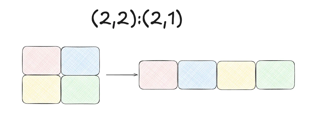
If we have a stride of $(2048, 1)$ we have that $L (x_{1} + 1, x_{2}) - L (x_{1}, x_{2}) = 2048$ and $L (x_{1}, x_{2} + 1) - L (x_{1}, x_{2}) = 1$ which means that two columns are adjacent in memory whereas two rows are "distant" in memory.

We could visualise that as follows:

Screenshot 2025-06-23 at 17

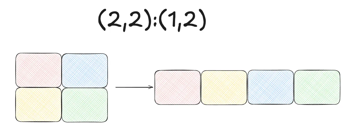
Similarly we could visualize the Layout where the entries in the stride are permutated:

Screenshot 2025-06-23 at 17

A layout like (2048, 2048):(2048,1) is frequently called row-major or in CuTe lingo K-major.

In our kernel we see the CuTe layout doing the job of obtaining the linear indexing for us.

# Map logical index to physical address via tensor layout
    a_val = gA[mi, ni]
    b_val = gB[mi, ni]

    # Perform element-wise addition
    gC[mi, ni] = a_val + b_val

When benchmarking with a matrix of size 32768 x 32768 this kernel archives 1936 GB/s on NVIDIA H100 80GB HBM3 using 256 threads per block.

Vectorised kernel

The kernel below performs

@cute.kernel
def vectorized_elementwise_add_kernel(
    gA: cute.Tensor,
    gB: cute.Tensor,
    gC: cute.Tensor,
):
    tidx, _, _ = cute.arch.thread_idx()
    bidx, _, _ = cute.arch.block_idx()
    bdim, _, _ = cute.arch.block_dim()

    thread_idx = bidx * bdim + tidx

    # Map thread index to logical index of input tensor
    m, n = gA.shape[1]  # thread-domain
    ni = thread_idx % n
    mi = thread_idx // n

    # Map logical index to physical address via tensor layout
    a_val = gA[(None, (mi, ni))].load()
    b_val = gB[(None, (mi, ni))].load()
    print(f"[DSL INFO] sliced gA = {gA[(None, (mi, ni))]}")
    print(f"[DSL INFO] sliced gB = {gB[(None, (mi, ni))]}")

    # Perform element-wise addition
    gC[(None, (mi, ni))] = a_val + b_val

It can be called as follows

@cute.jit
def vectorized_elementwise_add(mA: cute.Tensor, mB: cute.Tensor, mC: cute.Tensor):
    threads_per_block = 256

    gA = cute.zipped_divide(mA, (1, 4))
    gB = cute.zipped_divide(mB, (1, 4))
    gC = cute.zipped_divide(mC, (1, 4))

    print(f"[DSL INFO] Tiled Tensors:")
    print(f"[DSL INFO]   gA = {gA}")
    print(f"[DSL INFO]   gB = {gB}")
    print(f"[DSL INFO]   gC = {gC}")

    vectorized_elementwise_add_kernel(gA, gB, gC).launch(
        grid=(cute.size(gC, mode=[1]) // threads_per_block, 1, 1),
        block=(threads_per_block, 1, 1),
    )

When running this we can see in the terminal:

[DSL INFO] Tiled Tensors:
[DSL INFO]   gA = tensor<ptr<f16, gmem, align<16>> o ((1,4),(2048,512)):((0,1),(2048,4))>
[DSL INFO]   gB = tensor<ptr<f16, gmem, align<16>> o ((1,4),(2048,512)):((0,1),(2048,4))>
[DSL INFO]   gC = tensor<ptr<f16, gmem, align<16>> o ((1,4),(2048,512)):((0,1),(2048,4))>
[DSL INFO] sliced gA = tensor<ptr<f16, gmem, align<8>> o ((1,4)):((0,1))>
[DSL INFO] sliced gB = tensor<ptr<f16, gmem, align<8>> o ((1,4)):((0,1))>

This tell's us what is going on:

We simply tile the matrix along the columns, i.e. one thread handles 4 consecutive elements in memory. cute.size(gC, mode=[1]) // threads_per_block takes this accordingly into account, because we will launch 4 times less blocks for this kernel.

This tiling makes sense and will improve the performance of our kernel because GPUs are capable of 64B = 4 * 16B loads, i.e. we can load all 4 elements for the thread at once. This is a well known technique to improve performance in memory bound kernels. We choose the tiler to be (1, 4) because the original layout is N-major, i.e. the adjacent elements in memory are all in one column.

This kernel archives 3123 GB/s on NVIDIA H100 80GB HBM3 using 512 threads per block.

Use thread value layout

In more advanced CuTeDSL examples the concept of thread value layout is used heavily. It is therefore useful to study this concept more closely.

A kernel using thread value layout looks as follows:

@cute.kernel
def elementwise_add_kernel(
    gA: cute.Tensor, gB: cute.Tensor, gC: cute.Tensor, tv_layout: cute.Layout
):
    tidx, _, _ = cute.arch.thread_idx()
    bidx, _, _ = cute.arch.block_idx()

    # --------------------------------
    # slice for thread-block level view
    # --------------------------------
    blk_coord = ((None, None), bidx)

    # logical coord -> address
    blkA = gA[blk_coord]  # (TileM, TileN) -> physical address
    blkB = gB[blk_coord]  # (TileM, TileN) -> physical address
    blkC = gC[blk_coord]  # (TileM, TileN) -> physical address

    # --------------------------------
    # compose for thread-index & value-index to physical mapping
    # --------------------------------
    # blockA:    (TileM, TileN) -> physical address
    # tv_layout: (tid, vid)     -> (TileM, TileN)
    # tidfrgA = blkA o tv_layout
    # tidfrgA:   (tid, vid) -> physical address
    tidfrgA = cute.composition(blkA, tv_layout)
    tidfrgB = cute.composition(blkB, tv_layout)
    tidfrgC = cute.composition(blkC, tv_layout)

    print(f"Composed with TV layout:")
    print(f"  tidfrgA: {tidfrgA.type}")

    # --------------------------------
    # slice for thread-level view
    # --------------------------------
    # `None` represent slice of the entire per-thread data
    thr_coord = (tidx, None)

    # slice for threads: vid -> address
    thrA = tidfrgA[thr_coord]  # (V) -> physical address
    thrB = tidfrgB[thr_coord]  # (V) -> physical address
    thrC = tidfrgC[thr_coord]  # (V) -> physical address

    print(f"thrA/B/C:")
    print(f"  thrA: {thrA.type}")
    print(f"  thrB: {thrB.type}")
    print(f"  thrC: {thrC.type}")

    thrC[None] = thrA.load() + thrB.load()

The launch from the host side is as follows:

@cute.jit
def elementwise_add(
    mA: cute.Tensor,
    mB: cute.Tensor,
    mC: cute.Tensor,
):
    # mA layout: (M, N):(N, 1)
    # TV layout map thread & value index to (16, 256) logical tile
    #  - contiguous thread index maps to mode-1 because input layout is contiguous on
    #     mode-1 for coalesced load-store
    #  - each thread load 8 contiguous element each row and load 4 rows
    thr_layout = cute.make_layout((4, 32), stride=(32, 1))
    val_layout = cute.make_layout((4, 8), stride=(8, 1))
    tiler_mn, tv_layout = cute.make_layout_tv(thr_layout, val_layout)
    print(f"Tiler: {tiler_mn}")
    print(f"TV Layout: {tv_layout}")

    gA = cute.zipped_divide(mA, tiler_mn)  # ((TileM, TileN), (RestM, RestN))
    gB = cute.zipped_divide(mB, tiler_mn)  # ((TileM, TileN), (RestM, RestN))
    gC = cute.zipped_divide(mC, tiler_mn)  # ((TileM, TileN), (RestM, RestN))

    print(f"Tiled Input Tensors:")
    print(f"  gA: {gA.type}")
    print(f"  gB: {gB.type}")
    print(f"  gC: {gC.type}")

    # Launch the kernel asynchronously
    # Async token(s) can also be specified as dependencies
    elementwise_add_kernel(gA, gB, gC, tv_layout).launch(
        grid=[cute.size(gC, mode=[1]), 1, 1],
        block=[cute.size(tv_layout, mode=[0]), 1, 1],
    )

Running this will print out:

Tiler: (16, 256)
TV Layout: ((32,4),(8,4)):((128,4),(16,1))
Tiled Input Tensors:
  gA: !cute.memref<f16, gmem, align<16>, "((16,256),(128,8)):((2048,1),(32768,256))">
  gB: !cute.memref<f16, gmem, align<16>, "((16,256),(128,8)):((2048,1),(32768,256))">
  gC: !cute.memref<f16, gmem, align<16>, "((16,256),(128,8)):((2048,1),(32768,256))">
Composed with TV layout:
  tidfrgA: !cute.memref<f16, gmem, align<16>, "((32,4),(8,4)):((8,8192),(1,2048))">
thrA/B/C:
  thrA: !cute.memref<f16, gmem, align<16>, "((8,4)):((1,2048))">
  thrB: !cute.memref<f16, gmem, align<16>, "((8,4)):((1,2048))">
  thrC: !cute.memref<f16, gmem, align<16>, "((8,4)):((1,2048))">

We see that now we have a hierarchy in the tiling: BLOCK TILE -> THREAD TILE. TV layout is a map from the pairs (THREAD, VALUE) to the pair (TILE_M, TILE_N). The tiled layouts are a map from (TILE_M, TILE_N) to the physical address in memory. Therefore the composition of the to is a map from (THREAD, VALUE) to the physical address in memory. make_layout_tv will giv us the correct tiler_mn and tv_layout to obtain a valid map.

Let's take a closer look at thread and value layouts:

thr_layout = cute.make_layout((4, 32), stride=(32, 1))
val_layout = cute.make_layout((4, 8), stride=(8, 1))

Threads are organised into warps. A warp consists of 32 elements. Sequential memory accesses by threads within a warp can be grouped and executed as one. The above thread layout uses this fact and makes the threads within one warp sequential, i.e. they are next to each other in memory. In this way we organize a whole warp group, which is defined as the grouping of 4 warps.

The value layout reflects the fact that we load 8 sequential elements in one row. This can be done with an 8 * 16B = 128B load instruction. Each thread does this for 4 contiguous rows. This can be thought as a form of thread coarsening because we let each thread load multiple elements.

With the above setting this kernel archives 2960.80 GB/s. Note we could potentially apply Autotuning to improve performance, but I will stop at this point to keep the blog concise.

Conclusion

I hope the above block can explain some of the concepts behind CuTeDSL for CUDA programmers more accessible. For more tutorials please see the CuTeDSL example folder of the CUTLASS repo.